The Sharpe Ratio: Measuring Risk-Adjusted Returns

A 20% annual return sounds impressive until you learn it came with 50% drawdowns and sleepless nights. A 10% return sounds modest until you learn it arrived with minimal volatility and steady progress. Returns alone tell you what you made, but they don't tell you what you risked to make it. The Sharpe Ratio bridges this gap by measuring how much return you received for each unit of risk you took. This single number transforms how you evaluate investments, compare strategies, and understand whether strong performance came from skill or simply from taking on more risk than alternatives.

What the Sharpe Ratio reveals:

• The excess return earned above the risk-free rate per unit of volatility

• Whether an investment compensated you adequately for the risk involved

• How efficiently a portfolio or strategy converts risk into return

• A standardized way to compare investments with different risk profiles

• Which of two investments with similar returns actually performed better on a risk-adjusted basis

• Whether a manager's outperformance came from skill or from simply taking bigger bets

Why Returns Alone Mislead

Focusing solely on returns creates blind spots that can lead you toward riskier investments without realizing you're taking on that additional risk.

Two funds both return 15% annually over five years. Identical performance, right? Not if one achieved that return with steady monthly gains while the other swung wildly between 40% gains and 25% losses before arriving at the same destination. The steady fund let you sleep at night and stick with your investment plan. The volatile fund tested your discipline repeatedly and may have shaken you out at the worst possible moment. Raw returns treat these experiences as equivalent when they clearly aren't. The Sharpe Ratio captures this difference by penalizing returns that came with higher volatility, giving you a more complete picture of what the investment actually delivered relative to what it put you through.

What This Article Covers

This article explains how the Sharpe Ratio works, how to calculate and interpret it, and how to use it effectively while understanding its limitations.

Topics this article will cover:

• The formula behind the Sharpe Ratio and what each component represents

• How to interpret Sharpe Ratio values and what constitutes good, average, and poor readings

• The role of the risk-free rate and how it affects calculations

• Why standard deviation serves as the risk measure and when this assumption breaks down

• Practical applications for comparing funds, evaluating strategies, and constructing portfolios

• Limitations of the Sharpe Ratio and situations where it may mislead

• Alternative ratios like Sortino and Calmar that address some of the Sharpe Ratio's weaknesses

• Common mistakes investors make when using the Sharpe Ratio

The Sharpe Ratio measures risk-adjusted return by calculating how much excess return an investment generates for each unit of risk taken. "Excess return" means the return above what you could earn risk-free, typically represented by Treasury bills. "Risk" in this context means volatility, measured by standard deviation of returns. The ratio essentially asks: for every percentage point of volatility I accepted, how much additional return did I receive beyond the safe alternative? Higher ratios indicate more efficient conversion of risk into return, while lower ratios suggest the investment didn't adequately compensate for the volatility experienced.

William Sharpe and the Ratio's Origin

William F. Sharpe, a Nobel Prize-winning economist, introduced what he originally called the "reward-to-variability ratio" in 1966, and the financial industry later renamed it in his honor.

Sharpe developed the ratio while working on portfolio theory and the Capital Asset Pricing Model at the University of Washington and later Stanford. His insight was that investors shouldn't evaluate returns in isolation—they should evaluate returns relative to the risk required to achieve them. Before Sharpe's work, comparing a conservative bond fund to an aggressive stock fund based solely on returns made little sense because the comparison ignored the fundamentally different risk profiles. The Sharpe Ratio provided a standardized framework for these comparisons, enabling investors to ask whether the additional return from riskier investments justified the additional volatility. Sharpe received the Nobel Prize in Economics in 1990, partly for this contribution to financial theory.

The Concept of Risk-Adjusted Returns

Risk-adjusted returns acknowledge that earning 15% with low volatility represents fundamentally better performance than earning 15% with high volatility, even though the nominal returns are identical.

The concept rests on a simple premise: risk has a cost.

IF you can earn 8% with minimal volatility from a stable investment… THEN earning only 8% from a volatile investment represents poor compensation for the additional stress and uncertainty.

IF two investments both return 12% annually… THEN the one achieving that return with half the volatility delivered superior risk-adjusted performance.

IF a high-volatility strategy returns 20% while a low-volatility strategy returns 15%... THEN the Sharpe Ratio helps determine whether that extra 5% adequately compensated for the additional risk.

IF an investment's Sharpe Ratio is lower than a simple index fund's ratio… THEN you're taking on additional risk without receiving proportional additional return.

IF a manager claims exceptional performance based on high returns… THEN the Sharpe Ratio reveals whether those returns came from skill or simply from accepting more risk than benchmarks.

Why Risk Context Matters

Comparing investments without accounting for risk leads to decisions that feel rational but ignore important information about what you're actually buying.

Why raw return comparisons mislead:

• A fund returning 25% might have experienced 40% drawdowns while a fund returning 18% never dropped more than 12%

• High returns often come during periods of high risk-taking, which can reverse dramatically when conditions change

• Investors frequently abandon volatile investments during drawdowns, meaning they never actually capture the advertised long-term returns

• Leverage can artificially inflate returns while dramatically increasing risk, making comparisons to unleveraged investments meaningless

• Different asset classes have different baseline volatility levels, so comparing their raw returns ignores structural differences

• Past high returns from aggressive strategies often reflect favorable conditions that may not persist

• Two managers with identical returns but different volatility profiles have demonstrated very different skill levels

• The investment you can actually hold through difficult periods matters more than the investment with the highest theoretical return

The Bottom Line: The Sharpe Ratio provides a standardized measure of risk-adjusted returns by calculating excess return per unit of volatility, allowing meaningful comparisons between investments with different risk profiles and revealing whether strong returns came from genuine efficiency or simply from taking on more risk than alternatives.

The Sharpe Ratio formula is elegantly simple: subtract the risk-free rate from the investment's return, then divide by the standard deviation of returns. Written mathematically, it's (Rp - Rf) / σp, where Rp is the portfolio return, Rf is the risk-free rate, and σp is the standard deviation of the portfolio's returns. This formula produces a single number that captures how much excess return you earned for each unit of volatility you accepted. A ratio of 1.0 means you earned one percentage point of excess return for each percentage point of standard deviation—anything higher suggests increasingly efficient risk-to-return conversion.

The Three Components Explained

Each component of the Sharpe Ratio formula serves a specific purpose in measuring risk-adjusted performance.

The three components and what they represent:

• Portfolio return (Rp) is the total return of the investment over the measurement period, typically expressed as an annualized percentage

• This return includes all sources of gain: price appreciation, dividends, interest, and any other distributions

• The return should match the time period used for the other components—annual return with annual risk-free rate and annualized standard deviation

• Risk-free rate (Rf) represents the return available from a theoretically riskless investment, typically short-term Treasury bills

• Subtracting the risk-free rate isolates the "excess return"—the additional compensation received for taking risk beyond the safe alternative

• If an investment returns 10% but Treasury bills yield 4%, the excess return is only 6%

• Standard deviation (σp) measures the volatility of returns over the measurement period

• Higher standard deviation means returns varied more widely around the average—more uncertainty, more risk

• Standard deviation captures both upside and downside volatility, which represents both a feature and a limitation of the measure

• Using all three components together answers the question: how much return above the risk-free alternative did I earn per unit of volatility?

A Practical Calculation Example

Walking through a concrete example makes the formula tangible and shows how small differences in inputs can meaningfully change the resulting Sharpe Ratio.

Suppose you're evaluating a fund that returned 12% annually over the past five years, during which the average risk-free rate (using 3-month Treasury bills) was 2%, and the fund's annualized standard deviation was 15%. Plugging into the formula: (12% - 2%) / 15% = 10% / 15% = 0.67. This Sharpe Ratio of 0.67 tells you the fund earned 0.67 percentage points of excess return for each percentage point of volatility. Now compare this to a second fund that returned 10% with a standard deviation of only 8% during the same period: (10% - 2%) / 8% = 8% / 8% = 1.0. Despite lower absolute returns, the second fund has a higher Sharpe Ratio because it generated its excess return more efficiently. The first fund earned more in raw terms, but the second fund delivered better risk-adjusted performance. This comparison illustrates why the Sharpe Ratio matters—it reveals that the lower-returning fund actually did a better job converting risk into reward.

Once you've calculated a Sharpe Ratio, you need to know what the number actually means. Is 0.5 good? Is 1.5 exceptional? The answer depends on context, but general benchmarks exist to guide interpretation. Most practitioners consider ratios below 1.0 as suboptimal, ratios between 1.0 and 2.0 as good to very good, and ratios above 2.0 as excellent—though sustained ratios above 2.0 are rare and should prompt questions about whether the calculation period was unusually favorable or whether risks aren't being fully captured.

General Benchmarks and Guidelines

While no universal standard exists for what constitutes a "good" Sharpe Ratio, the investment industry has developed rough guidelines through decades of practical application.

Common interpretation benchmarks:

• Below 0: The investment returned less than the risk-free rate, meaning you took risk and weren't compensated for it at all

• 0 to 0.5: Subpar risk-adjusted returns that generally don't justify the volatility experienced

• 0.5 to 1.0: Acceptable but not impressive—the investment generated some excess return per unit of risk but nothing exceptional

• 1.0 to 2.0: Good to very good risk-adjusted performance, indicating efficient conversion of risk into return

• 2.0 to 3.0: Excellent performance that's difficult to sustain over long periods

• Above 3.0: Exceptional and rare—should prompt investigation into whether the measurement period was unusually favorable or risks are understated

• The S&P 500 has historically produced Sharpe Ratios between 0.4 and 0.6 over long periods, providing a useful benchmark for equity investments

• Bond portfolios typically show Sharpe Ratios between 0.2 and 0.5 due to lower excess returns despite also having lower volatility

• Hedge funds and active managers often target Sharpe Ratios above 1.0 to justify their fees and complexity

Context Matters in Interpretation

A Sharpe Ratio doesn't exist in a vacuum—the same number can represent strong or weak performance depending on the investment type, market conditions, and comparison set.

A Sharpe Ratio of 0.8 for an aggressive small-cap growth fund might represent excellent risk-adjusted performance given the asset class's inherent volatility, while the same 0.8 for a conservative balanced fund might indicate disappointing efficiency. Market conditions during the measurement period matter enormously. Bull markets tend to produce higher Sharpe Ratios across most investments because returns are elevated while volatility often remains contained. Bear markets and volatile periods compress Sharpe Ratios even for well-managed portfolios. Comparing a fund's Sharpe Ratio to its relevant benchmark and peer group provides more useful information than evaluating the number in isolation. A fund with a 0.7 Sharpe Ratio that consistently exceeds its benchmark's 0.5 ratio is adding value, while a fund with a 1.2 Sharpe Ratio that trails its benchmark's 1.5 ratio is underperforming despite the seemingly strong absolute number.

Remember: The Sharpe Ratio gains meaning through comparison rather than in isolation—evaluate ratios against relevant benchmarks, peer groups, and the specific asset class's typical range, while recognizing that market conditions during the measurement period heavily influence results and that exceptionally high ratios warrant skepticism about sustainability or hidden risks.

The risk-free rate represents the return you could earn without taking any risk—the baseline against which all risky investments are measured. By subtracting this rate from an investment's return, the Sharpe Ratio isolates the excess return attributable to accepting risk. If you could earn 5% from Treasury bills with essentially zero volatility, then an investment returning 8% has only generated 3% of excess return. The remaining 5% wasn't compensation for risk—it was simply what money earned by existing. This distinction matters because it prevents investors from confusing baseline returns available everywhere with genuine alpha generated through accepting volatility.

What Qualifies as Risk-Free

No investment is truly risk-free, but certain instruments come close enough that finance treats them as proxies for the theoretical riskless rate.

Common risk-free rate proxies:

• U.S. Treasury bills (T-bills) with maturities of 3 months or less serve as the most common proxy

• T-bills are backed by the U.S. government's ability to tax and print currency, making default essentially impossible

• Short maturities minimize interest rate risk, meaning the bills return almost exactly their stated yield

• The 3-month T-bill rate is the most widely used risk-free rate in Sharpe Ratio calculations

• Some practitioners use 1-month T-bills for even shorter duration exposure

• The 10-year Treasury yield is sometimes used but introduces interest rate risk that technically violates the risk-free concept

• LIBOR and its replacement rates (SOFR) were historically used but include small credit risk premiums

• For international investments, local government short-term securities may serve as the appropriate risk-free proxy

• Money market fund yields approximate the risk-free rate but include minimal credit and liquidity risk

How Changing Rates Affect the Ratio

The risk-free rate isn't static, and its movements directly impact Sharpe Ratio calculations even when investment performance remains constant.

The risk-free rate changes over time based on Federal Reserve policy, inflation expectations, and economic conditions.

IF the risk-free rate rises while your investment return stays constant… THEN your excess return shrinks and your Sharpe Ratio declines, even though your actual investment performance hasn't changed.

IF the risk-free rate falls toward zero as it did during 2009-2021… THEN excess returns expand and Sharpe Ratios rise across most investments, flattering performance during that era.

IF you compare Sharpe Ratios from different interest rate environments without adjustment… THEN you may incorrectly conclude that performance during low-rate periods was superior to high-rate periods.

IF you're evaluating a fund's historical Sharpe Ratio spanning decades… THEN recognize that varying risk-free rates across that period affected the calculation throughout.

IF rates rise significantly from recent lows… THEN many investments that showed strong Sharpe Ratios during the low-rate era will see their ratios compress going forward.

Adjusting for Different Time Periods

Consistency in time period matching between returns, risk-free rates, and standard deviation is necessary for meaningful Sharpe Ratio calculations.

The Sharpe Ratio requires that all three components—return, risk-free rate, and standard deviation—use the same time period. If you're calculating an annualized Sharpe Ratio, you need annualized return, an annual risk-free rate, and annualized standard deviation. Monthly returns require monthly risk-free rates and monthly standard deviation. Mixing periods creates mathematical errors that produce meaningless results. When annualizing from shorter periods, returns and risk-free rates typically multiply by the number of periods per year (monthly returns times 12), while standard deviation multiplies by the square root of the number of periods (monthly standard deviation times the square root of 12). Using average risk-free rates over your measurement period rather than a single point-in-time rate provides a more accurate picture of the opportunity cost throughout the investment horizon.

Quick tip: When comparing Sharpe Ratios across different time periods, note the prevailing risk-free rate during each period—a ratio of 1.0 when T-bills yielded 5% represents different absolute performance than a ratio of 1.0 when T-bills yielded 0.5%.

Quick tip: For most retail investor applications, using the average 3-month T-bill rate during your measurement period provides a reasonable and widely accepted risk-free rate proxy for Sharpe Ratio calculations.

The Sharpe Ratio uses standard deviation as its measure of risk, equating volatility with uncertainty and uncertainty with risk. Standard deviation quantifies how widely returns scatter around their average—a high standard deviation means returns varied dramatically from period to period, while a low standard deviation means returns clustered tightly around the mean. This choice of risk measure has both logical appeal and significant limitations that users should understand before relying on the Sharpe Ratio for important decisions.

Why volatility serves as the risk proxy:

• Standard deviation captures the unpredictability of returns, reflecting the range of outcomes an investor might experience

• Higher volatility creates larger drawdowns that test investor discipline and may force selling at inopportune times

• Volatile investments are harder to plan around for retirees or those with specific liquidity needs

• Standard deviation is mathematically convenient, well-understood, and easy to calculate from historical return data

• The measure aligns with modern portfolio theory's treatment of variance as the primary risk factor

• For normally distributed returns, standard deviation provides a complete picture of the return distribution's shape

• Volatility correlates with the emotional experience of investing—high-volatility investments feel riskier even when long-term outcomes are similar

• The measure allows comparison across different asset types using a common scale

Calculating Standard Deviation of Returns

Standard deviation calculation follows a specific process that measures the average distance of each return from the mean return.

To calculate standard deviation of returns, start by computing the average return over your measurement period. Then, for each period's return, calculate the difference from that average and square it—squaring eliminates negative values and emphasizes larger deviations. Sum all these squared differences and divide by the number of periods minus one (for sample standard deviation) or by the number of periods (for population standard deviation). Finally, take the square root of this result to return to the original units of measurement. For annualized standard deviation from monthly data, multiply the monthly standard deviation by the square root of 12. Most financial software and spreadsheets automate this calculation, but understanding the underlying process helps you recognize what the number actually represents—the typical deviation from average returns that you should expect to experience.

Limitations of Standard Deviation

Using standard deviation as the sole risk measure introduces blind spots that the Sharpe Ratio inherits by design.

DO recognize that standard deviation treats upside and downside volatility identically, penalizing investments that occasionally surge higher.

DO understand that standard deviation assumes returns follow a normal distribution, which real-world returns often violate.

DO acknowledge that two investments with identical standard deviations can have very different risk profiles if one has fat tails or skewed returns.

DO consider that standard deviation measures historical volatility, which may not predict future volatility during regime changes.

DON'T assume a low standard deviation means an investment is safe—it may simply reflect a quiet period before a large loss.

DON'T ignore that standard deviation doesn't capture liquidity risk, credit risk, or concentration risk that may matter greatly.

DON'T forget that standard deviation measured over short periods may understate true long-term risk by missing rare events.

DON'T rely solely on the Sharpe Ratio for investments with non-normal return distributions like options strategies or distressed debt.

When Volatility Misses True Risk

Certain investment characteristics create situations where standard deviation fails to capture the actual risks involved, making the Sharpe Ratio potentially misleading.

Strategies that sell options or provide insurance-like payoffs often show low standard deviation and attractive Sharpe Ratios during normal conditions because they collect steady premium income without apparent volatility. But these strategies carry tail risk—the possibility of large, sudden losses when rare events occur. Their standard deviation understates risk because the data sample may not include the catastrophic scenario that eventually arrives. 

Similarly, illiquid investments like private equity or real estate may report smooth returns not because volatility is genuinely low but because the assets aren't marked to market frequently. Their Sharpe Ratios appear favorable due to understated volatility rather than superior risk-adjusted performance. Investments with leverage, concentrated positions, or exposure to binary outcomes may also display misleading Sharpe Ratios because their primary risk—the possibility of severe loss—doesn't show up in period-to-period standard deviation until the event actually occurs.

Keep In Mind: The Sharpe Ratio's use of standard deviation as the risk measure works well for diversified portfolios with relatively normal return distributions, but creates blind spots for strategies with tail risk, illiquid assets with smoothed returns, or investments where upside volatility differs meaningfully from downside volatility—recognizing these limitations helps you know when to supplement the Sharpe Ratio with alternative risk measures.

The Sharpe Ratio moves from theoretical concept to practical tool when you apply it to real investment decisions. Whether you're selecting mutual funds, evaluating your own trading system, building a portfolio, or assessing whether a manager deserves their fees, the ratio provides a standardized framework for comparing risk-adjusted performance. The key is applying it consistently across comparable investments while recognizing when the comparison makes sense and when other factors should dominate your decision.

Comparing Mutual Funds and ETFs

The Sharpe Ratio excels at comparing funds within the same category, revealing which managers convert risk into return most efficiently.

How to use the Sharpe Ratio for fund comparison:

• Compare funds within the same category—large-cap growth to large-cap growth, not large-cap growth to short-term bonds

• Look for funds with higher Sharpe Ratios than their category average over meaningful time periods of three to five years

• A fund with a lower absolute return but higher Sharpe Ratio may be a better choice for risk-conscious investors

• Compare each fund's Sharpe Ratio to its benchmark index to determine whether active management adds value

• Index funds provide a useful baseline—if an active fund can't exceed the index's Sharpe Ratio, you're paying fees for nothing

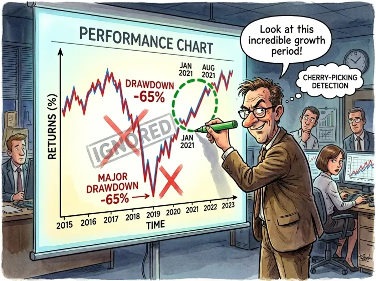
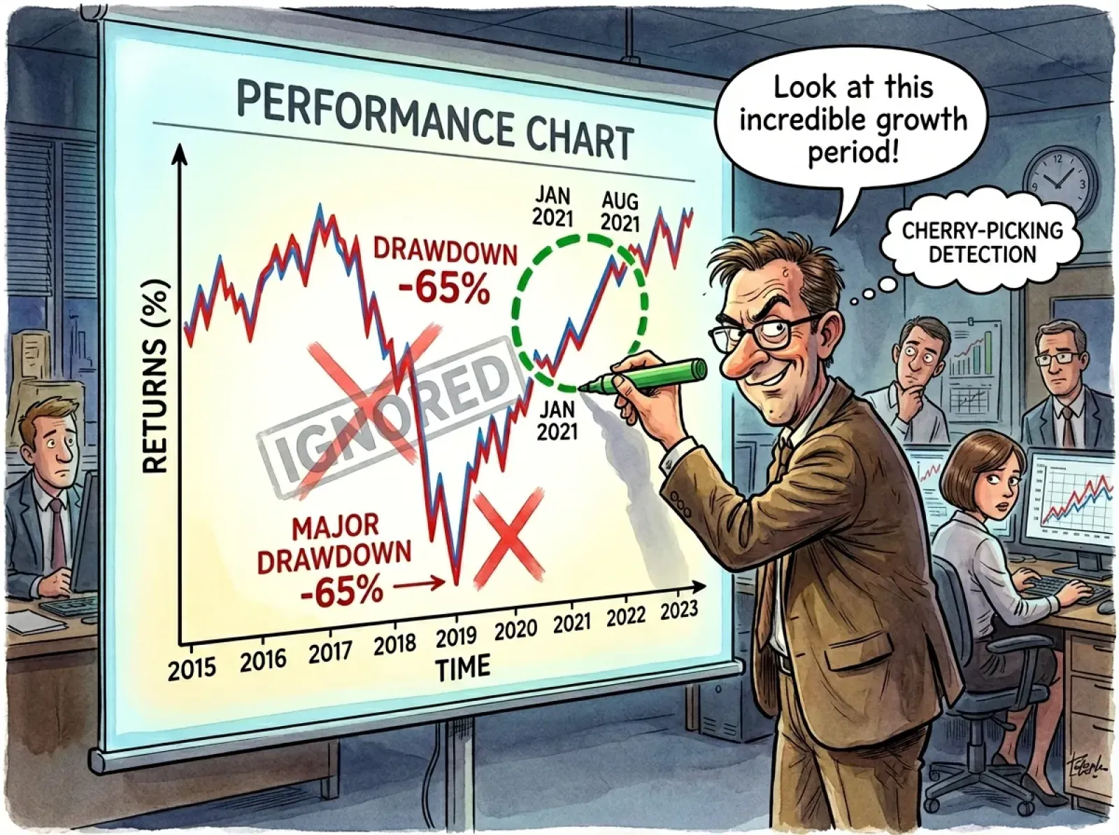
• Consider Sharpe Ratios across multiple time periods rather than cherry-picking favorable windows

• Two funds with similar Sharpe Ratios but different volatility levels may suit different investor temperaments

• Higher expense ratios reduce returns without reducing volatility, mechanically lowering Sharpe Ratios over time

Evaluating Trading Strategies

Whether you're developing your own trading system or evaluating someone else's claimed results, the Sharpe Ratio provides a reality check on performance claims.

Questions to ask when evaluating strategy Sharpe Ratios:

• What time period produced this Sharpe Ratio, and does it include both favorable and unfavorable market conditions?

• Is the Sharpe Ratio calculated from live trading results or backtested simulations that may be overfit to historical data?

• Does the strategy's return distribution match the assumptions underlying the Sharpe Ratio, or does it carry tail risks that standard deviation misses?

• How does the strategy's Sharpe Ratio compare to a simple benchmark approach requiring no active management?

• Would transaction costs, slippage, and taxes reduce the actual achievable Sharpe Ratio below the theoretical calculation?

• Has the Sharpe Ratio remained consistent across different market regimes, or does it depend on specific conditions persisting?

• If the Sharpe Ratio seems exceptionally high (above 2.0), what risks might be understated or what data mining might have occurred?

• Can the strategy scale to meaningful position sizes without degrading its Sharpe Ratio through market impact?

Portfolio Construction and Manager Evaluation

The Sharpe Ratio informs portfolio construction by helping you allocate capital toward the most efficient risk-adjusted opportunities and evaluate whether managers justify their compensation.

When constructing portfolios, the Sharpe Ratio helps identify which investments contribute the most return per unit of risk added. A portfolio consisting entirely of the highest-return assets isn't necessarily optimal if those assets also carry the highest volatility. Adding a lower-return, lower-volatility asset might improve the portfolio's overall Sharpe Ratio if it provides diversification benefits. For manager evaluation, the Sharpe Ratio cuts through marketing claims and reveals whether outperformance came from genuine skill or simply from taking bigger risks than the benchmark. A manager who consistently beats the benchmark but does so with proportionally higher volatility hasn't demonstrated skill—they've demonstrated willingness to accept more risk. The Sharpe Ratio identifies managers who deliver excess returns without proportionally higher volatility, which suggests genuine alpha generation rather than beta loading.

Think of it this way: The Sharpe Ratio serves as a common language for comparing investments that would otherwise be apples to oranges—whether you're choosing between mutual funds, testing trading strategies, building diversified portfolios, or evaluating whether a manager's fees are justified by their risk-adjusted performance rather than just their raw returns.

No single metric captures everything, and the Sharpe Ratio is no exception. Understanding its limitations prevents over-reliance on a number that provides useful but incomplete information. The ratio works well for comparing diversified portfolios with reasonably normal return distributions over consistent time periods. It works less well for strategies with asymmetric payoffs, investments with tail risks, or comparisons across different market environments. Recognizing when the Sharpe Ratio applies cleanly versus when it may mislead helps you use it as one tool among many rather than the final word on investment quality.

Limitations to recognize when using the Sharpe Ratio:

• Assumes returns follow a normal distribution, but real-world returns often exhibit fat tails with more extreme outcomes than normal distributions predict

• Many investment strategies produce skewed returns that deviate significantly from the bell curve the ratio implicitly assumes

• Treats upside volatility and downside volatility identically, penalizing investments that occasionally produce large gains

• An investment that rarely loses money but occasionally surges may show a lower Sharpe Ratio than its actual risk profile warrants

• Most investors care far more about downside volatility than upside volatility, yet the ratio weights them equally

• Highly sensitive to time period selection, with different measurement windows producing dramatically different ratios for the same investment

• Cherry-picking favorable time periods can make mediocre investments appear exceptional and vice versa

• Short measurement periods produce unreliable ratios that may not reflect true long-term risk-adjusted performance

• Doesn't capture tail risk—the possibility of rare but severe losses that standard deviation fails to measure

• Strategies that sell options or provide insurance-like returns often show artificially high Sharpe Ratios until the tail event occurs

• Illiquid investments may report smoothed returns that understate true volatility, inflating their Sharpe Ratios

• The ratio can't distinguish between skill and luck over short time periods

• Changing risk-free rates across measurement periods affect comparisons between different eras

• Transaction costs, taxes, and implementation friction reduce actual achievable Sharpe Ratios below calculated values

• The ratio provides no information about drawdown magnitude, recovery time, or sequence of returns

• Leverage can artificially manipulate Sharpe Ratios in ways that obscure underlying strategy quality

When to Look Beyond the Sharpe Ratio

Certain investment types and situations require supplementing the Sharpe Ratio with alternative measures that address its specific blind spots.

When evaluating investments with asymmetric return profiles—options strategies, venture capital, distressed debt, or insurance-like payoffs—the Sharpe Ratio's assumption of normal distributions and equal treatment of upside and downside volatility creates meaningful distortions. For these investments, consider ratios like Sortino (which focuses only on downside deviation), Calmar (which incorporates maximum drawdown), or analysis of the full return distribution including skewness and kurtosis. For investments where tail risk matters significantly, stress testing and scenario analysis reveal information the Sharpe Ratio cannot provide.

The Bottom Line: The Sharpe Ratio provides valuable information for comparing diversified investments with reasonably normal return distributions, but its assumptions about normality, equal treatment of upside and downside volatility, sensitivity to time periods, and inability to capture tail risk mean it should serve as one input among many rather than the sole determinant of investment quality—and recognizing these limitations helps you know when to trust the ratio and when to supplement it with other analysis.

The Sharpe Ratio's limitations have inspired alternative metrics that address specific weaknesses while preserving the core concept of risk-adjusted returns. Each alternative modifies how "risk" is defined or measured, providing different perspectives on the same underlying question: did this investment adequately compensate me for the risks I accepted? Understanding these alternatives helps you select the right tool for each evaluation context and build a more complete picture of risk-adjusted performance than any single metric provides.

Sortino Ratio for Downside Focus

The Sortino Ratio addresses one of the Sharpe Ratio's most criticized limitations by measuring only downside volatility rather than total volatility.

Key characteristics of the Sortino Ratio:

• Formula replaces standard deviation with downside deviation, measuring only returns below a target or minimum acceptable return

• Upside volatility—those pleasant surprises when investments surge higher—doesn't penalize the ratio

• Better reflects how most investors actually experience risk, since losses create stress while gains create satisfaction

• Particularly useful for investments with asymmetric return profiles where upside potential differs meaningfully from downside risk

• A higher Sortino Ratio indicates better return per unit of downside risk specifically

• The target return used in the denominator can be zero, the risk-free rate, or any minimum acceptable return threshold

• Sortino Ratios tend to be higher than Sharpe Ratios for investments with more upside than downside volatility

• The ratio struggles with investments that rarely produce negative returns, potentially producing unstable or misleading values

Calmar Ratio for Drawdown Consideration

The Calmar Ratio replaces volatility entirely with maximum drawdown, focusing on the worst peak-to-trough decline an investor would have experienced.

For investors who care most about capital preservation and avoiding deep losses, maximum drawdown may matter more than period-to-period volatility. An investment that fluctuates modestly but once dropped 60% carries different risk than one with higher monthly volatility that never declined more than 20%. The Calmar Ratio captures this distinction by dividing annualized return by maximum drawdown. A Calmar Ratio of 1.0 means the annual return equals the maximum drawdown—you earned as much per year as you would have lost during the worst decline. Higher ratios indicate better return relative to the worst-case experience. The ratio is particularly popular among hedge fund evaluators and commodity trading advisors who prioritize drawdown management. Its limitation is sensitivity to the measurement period—a longer period typically includes more severe drawdowns, mechanically lowering the ratio.

Information Ratio for Benchmark Comparison

The Information Ratio measures excess return relative to a benchmark, divided by the tracking error (standard deviation of the difference between portfolio and benchmark returns).

When to use the Information Ratio:

• Evaluating active managers against their stated benchmarks rather than against the risk-free rate

• Determining whether a manager's deviation from the benchmark produced commensurate excess returns

• Comparing managers who use the same benchmark but take different levels of active risk

• Assessing whether paying active management fees is justified by benchmark-relative performance

• A ratio above 0.5 is generally considered good; above 1.0 is excellent

• The ratio answers a specific question: did active bets pay off relative to how much active risk was taken?

• Less useful for absolute return strategies without clear benchmarks

• Complements rather than replaces the Sharpe Ratio, providing benchmark-relative context alongside absolute risk-adjusted performance

Pro tip: Use the Sortino Ratio alongside the Sharpe Ratio when evaluating investments where you specifically care about downside protection—comparing the two ratios reveals whether an investment's volatility comes primarily from upside moves (Sortino much higher than Sharpe) or downside moves (ratios similar).

Pro tip: When evaluating managers or strategies with explicit drawdown limits or capital preservation mandates, the Calmar Ratio often provides more relevant information than the Sharpe Ratio because it directly measures what those strategies are designed to control.

The Sharpe Ratio is simple enough to calculate but easy to misuse. Mistakes in application undermine the ratio's value and can lead to poor investment decisions based on misleading comparisons. Most errors fall into predictable categories: manipulating the measurement period, making inappropriate comparisons, forgetting the ratio's assumptions, or treating the number as more meaningful than it actually is. Avoiding these mistakes helps you extract genuine insight from the ratio rather than false confidence.

Common mistakes when using the Sharpe Ratio:

• Cherry-picking favorable time periods that make investments look better than their full track record would suggest

• Presenting a five-year Sharpe Ratio that conveniently starts after a major drawdown or ends before one

• Comparing ratios calculated over different time periods without acknowledging the inconsistency

• Comparing Sharpe Ratios across fundamentally different asset classes that have different baseline volatility characteristics

• Expecting a bond fund's Sharpe Ratio to match an equity fund's without recognizing structural differences

• Comparing an emerging market fund to a Treasury fund as if the ratios should be similar

• Ignoring that the ratio assumes normally distributed returns when evaluating strategies with fat tails or skewed payoffs

• Trusting high Sharpe Ratios from options-selling strategies or other insurance-like approaches without stress testing

• Forgetting that illiquid investments may show artificially high ratios due to smoothed or stale pricing

• Over-relying on a single metric to make complex investment decisions that involve multiple risk dimensions

• Ignoring qualitative factors like manager experience, organizational stability, or strategy capacity

• Failing to consider maximum drawdown, correlation, liquidity, or other risk factors the Sharpe Ratio doesn't capture

• Using short time periods that produce unreliable ratios with high statistical noise

• Treating backtested Sharpe Ratios as equivalent to live trading results despite potential overfitting

• Failing to account for fees, transaction costs, and taxes that reduce actual achievable ratios

• Assuming a high historical Sharpe Ratio guarantees future performance

• Ignoring regime changes that may make historical ratios irrelevant going forward

Avoiding These Mistakes

Sound Sharpe Ratio analysis requires consistency, appropriate comparisons, awareness of assumptions, and integration with other information rather than blind reliance on a single number.

Use consistent, meaningful time periods that include both favorable and unfavorable market conditions—ideally spanning at least one full market cycle. Compare investments only within the same asset class or strategy category where baseline risk characteristics are similar. Remember the ratio's assumptions and supplement with alternative metrics when evaluating investments with non-normal return distributions or significant tail risks. Treat the Sharpe Ratio as one input among many, combining it with drawdown analysis, qualitative assessment, and other risk measures to build a complete picture.

The Bottom Line: The Sharpe Ratio becomes misleading when users cherry-pick favorable time periods, make comparisons across incompatible asset classes, ignore the ratio's assumptions about return distributions, or treat it as the sole determinant of investment quality—avoiding these common mistakes means using consistent measurement periods, comparing within appropriate peer groups, recognizing when assumptions don't hold, and integrating the ratio with other risk measures for complete analysis.

The Sharpe Ratio offers something valuable: a standardized way to ask whether an investment compensates you adequately for the risk involved. This question matters because returns alone tell an incomplete story. Two investments with identical returns but different volatility profiles delivered fundamentally different experiences, and the Sharpe Ratio captures that difference in a single comparable number. Once you understand how to calculate the ratio, interpret its values, and recognize its limitations, you have a tool that improves decision-making across fund selection, strategy evaluation, portfolio construction, and manager assessment.

Beyond the Numbers

The Sharpe Ratio works best as one component of a broader analytical framework that combines quantitative metrics with qualitative judgment and common sense.

No single number, however well-constructed, captures everything that matters about an investment. The Sharpe Ratio tells you about historical risk-adjusted returns but not about the people managing the money, the sustainability of the strategy, the potential for future regime changes, or the fit between the investment and your specific goals. Use the ratio to screen and compare, but don't let it replace deeper analysis. A fund with a slightly lower Sharpe Ratio but a more experienced team, more transparent process, and better alignment with your needs may be the superior choice. Similarly, a strategy with an impressive historical Sharpe Ratio may have achieved that record under conditions that no longer apply. The goal isn't to optimize for the highest Sharpe Ratio but to make risk-adjusted thinking a natural part of how you evaluate opportunities—asking not just "what did it return?" but "what did it return relative to the risk required?" This shift in perspective, more than any specific calculation, represents the lasting value of understanding the Sharpe Ratio.